Crushable Foam Series: Exploring Material Models in Simple Test Cases - Compression

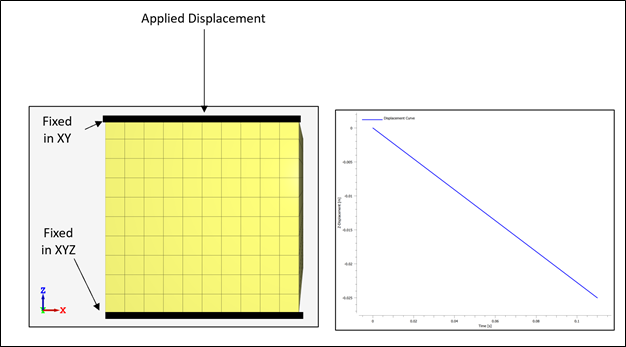
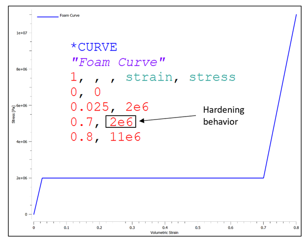
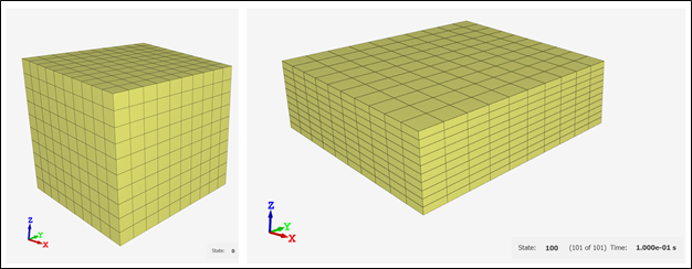
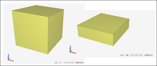
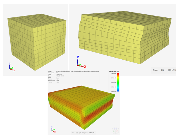
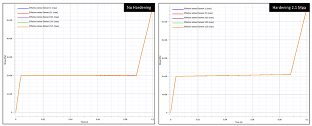
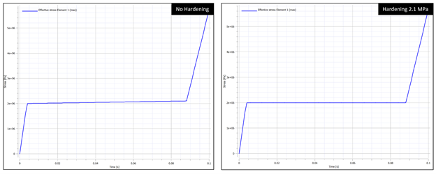
     In the coming weeks, I will be writing a few articles that explore the importance of understanding and checking basic components of finite element models, particularly when dealing with any form of nonlinearity, including material nonlinearity, geometric nonlinearity, or contact nonlinearity. The goal of these articles is to explore key components of finite element analysis using simple models whose concepts apply and propagate to larger scale models and systems. All models in this series are built using the IMPETUS Afea Solver®, an explicit nonlinear transient dynamic finite element solver. The use of this solver allows for such studies and analysis to be performed efficiently and intuitively due to its use of parameters, in-built geometry options, mesh commands, and unique element formulation.
     To kick off this series, we will first examine a simple uniaxial compression test of crushable foam. In this discussion, we will be exploring the importance of accurate material models, the effects of mesh density on model response, and numerical stability in explicit models.
        This model consists of a 50mm x 50mm x 50mm cube fixed at the bottom face in XYZ translational degrees of freedom and fixed at the top face in XY translational degrees of freedom. Note that solids do not support rotation at nodes, so rotational degrees of freedom are not constrained. A displacement that is linearly ramped over a time of 0.1 seconds is applied to the top face in the Z direction, causing uniform axial compression of the foam. Both the constraints and displacement were applied using the *BC_MOTION command. Illustrations of the model setup, including boundary conditions and geometry, and the applied displacement are shown in Figure 1. The model shown consists of 10x10x10 linear elements, however, additional models were run with 5x5x5 linear elements and a single linear element. A single model was also tested using a solution time of 1 second to ensure that the shorter solution time could approximate a quasi-static solution and did not induce inertial effects. 

Figure 1. Model setup and displacement curve.

    ​The cube was constructed of a representative model of aluminum crushable foam using *MAT_FOAM. A Poisson ratio of 0 was used and the stress-volumetric strain curve for the model is shown below in Figure 2. Note that this curve is purely representational and not taken from actual material test data. If a material model were being used in a larger finite element model, accurate material data would need to be obtained through testing or a viable material database to properly calibrate/validate the model. Additional calibration may also need to include geometry similar to the end-use case. Note that for crushable foam, there is an initial period of elastic yield, a constant stress compression, followed by foam densification where the stress increases. In an "ideal" case, no hardening would be present (i.e. the central curve would be flat). The lack of hardening, however, presents numerical issues and the global model response dependence on material hardening will be explored. As such, two foam material models were used in this study, one with no hardening (i.e. a flat central curve) and one with hardening (i.e. minor slope to central curve). This was accounted for by modifying the value of the y-coordinate of the third point in the curve definition as shown in Figure 2.

Figure 2. Stress vs. volumetric strain for representative *MAT_FOAM material model.

     Table 1 outlines the cases explored in this initial study, including number of elements, element order, presence of hardening, and y-coordinates for the start and end point of hardening behavior (all x-coordinates occur at 0.7). The key metric assessed in this model is effective stress and its relationship to mesh density and hardening. Later studies will explore element order and strain rate for uniaxial compression cases and punch cases.
     It is important to note that IMPETUS is an explicit solver, meaning that solutions are conditionally stable (numerical stability not guaranteed like in implicit models), and inputs and outputs must be checked carefully to ensure that the behavior makes physical sense. As is usually the case in numerical methods, your outputs are only as good as your inputs - “garbage in = garbage out." Accurate material models, mesh density, and element type/order are of particular importance, in addition to intuitive sanity checks that verify the material response is what would be expected based on physics of the problem. Note also that IMPETUS does not use shell elements and the number of element types are significantly reduced, allowing for variability due to selected element type to be significantly reduced. 

Table 1. Test cases explored in initial study.

Figures 3, 4, and 5 illustrate the anticipated deformation responses of a uniaxial compression model for crushable foam with minimal Poisson effect. Figure 3 corresponds to case 3 (with hardening), Figure 4 corresponds to Cases 4 and 5 (with and without hardening), and Figure 5 corresponds to cases 6 and 7 (with and without hardening). Note that the cube compresses uniformly and does not exhibit lateral expansion when numerically stable. Also note that this response was seen at lower mesh densities with and without hardening. 

Figure 3. Anticipated deformation response of 10x10x10 model with hardening.

Figure 4. Anticipated deformation response of 5x5x5 model with and without hardening.

Figure 5. Anticipated deformation response of single element model with and without hardening.

     Figure 6 shows the deformation response and effective stress response for the 10x10x10 model without hardening (Case 1 and 2). Figure 7 further illustrates the effective stress in various elements of the 10x10x10 model with varying hardening parameters (2.0 Mpa, 2.05 Mpa, and 2.1 Mpa). 

Figure 6. Deformation and stress response for 10x10x10 model without hardening.

Figure 7. Effective stress response of 10x10x10 model with and without hardening in the material model definition.

     Note the nonuniform stress response and outward bowing/bending in the model. Given the boundary conditions and understanding of the physics of the problem, this solution seems unlikely to be physical. Furthermore, this stress response was dependent on mesh density and was seen when the mesh density was increased to 10x10x10, but not observed in the global deformation response at lower element densities. Observing this kind of model response is usually indicative of some form of numerical instability, particularly when dealing with explicit solvers.
     One can see that, for the 10x10x10 model, spurious stresses develop when there is no hardening (a flat curve), that the magnitude and dispersion of these stresses decreases when the hardening is increased to 2.05 Mpa, and that the effect is fully eliminated when the hardening is increased to 2.1 Mpa. The convergence of the element response to the defined material behavior confirms this. This particular observation and phenomenon, that spurious stresses develop at varying mesh densities and varying material curve input, illustrates the importance of validating a material model prior to using it in full scale simulations. It is key to ensure that the material response that is observed matches the input for simple test cases that reflect the use cases in order to avoid the propagation of non-physical responses into larger models. This is typically done by modifying relevant parameters in the material model until the model response matches the test data gathered.
     The dependence of the response on mesh density can be further observed in Figures 8 and 9. While the global response in the 5x5x5 model did not show instability visually, minor instabilities can be observed in the plots of the stress responses without hardening These instabilities are also eliminated when hardening is added. No instabilities are seen in the single element model.  

Figure 8. Effective stress response for 5x5x5 model with and without hardening.

Figure 9. Effective stress response for single element model with and without hardening.

     In this particular case, the cause of the instability and unanticipated stress response was the need to add hardening behavior to the material model. In other situations in which there is test data available, other parameters may need to be modified to achieve the desired result. Additionally, it was seen that mesh density affected the response of the foam, bringing up another key point on response convergence. Performing mesh sensitivity or convergence studies when performing analysis is key to ensuring you are accurately capturing the full response of your system. If the model stress response changes significantly with changes in mesh density, it is likely that the mesh is not detailed enough to capture the response. Sensitivity studies, in general, are good tools to explore the stability of models. It may be necessary, additionally, to consider validating a material model with test data at a specified, set mesh density that allows for the simulation to solve in reasonable time frames. Explicit modeling presents some challenges due to solution time and accuracy depending on the size of the smallest element in the model. As usual, there is a fine line to walk between required model accuracy and computational time. 
     Through this simple example, we can see that the base components of finite element models - the simple things such as mesh density and material model - are incredibly important when building an analysis model and in ensuring that the results and response are accurate and reflective of the physical behavior.
      While this example is very simple and explores only a few parameters, there are a few key take-aways:

• Explicit models are conditionally stable, and we must pay careful attention to the responses to ensure there are no numerical instabilities or non-physical responses
• Mesh sensitivity and convergence studies are necessary to ensure the response converges 
• Sensitivity studies can be used in general to explore model stability and relative influence of system parameters 
• Material models should be validated prior to use in analysis with real-world test data